2023.September ~ 2023.December
In recent years, there have been notable progressions in autonomous vehicle technology. With the ongoing development and testing of an expanding number of self-driving vehicles, there is a growing demand for reliable controllers and effective algorithms for path planning. This is essential to guarantee the safety and dependability of autonomous operations.
The objective of the project is to construct different types of controllers, i.e. PID, pole placement, LQR and Kalmen filter to control the Tesla 3 autonomous vehicle and also Dji in python webots setting. In particular, the longitudinal and lateral controllers are needed for controlling the speed and orientation of the vehicle.
The performance of vehicle improves by utilizing different types of controllers and tuning of parameters.
The car drives around a track with the same geometry as the CMU buggy course. Buggy is a time-honored CMU tradition where students race human-powered, small, aerodynamic vehicles around Schenley Park's Flagstaff Hill. More information on it can be found here.
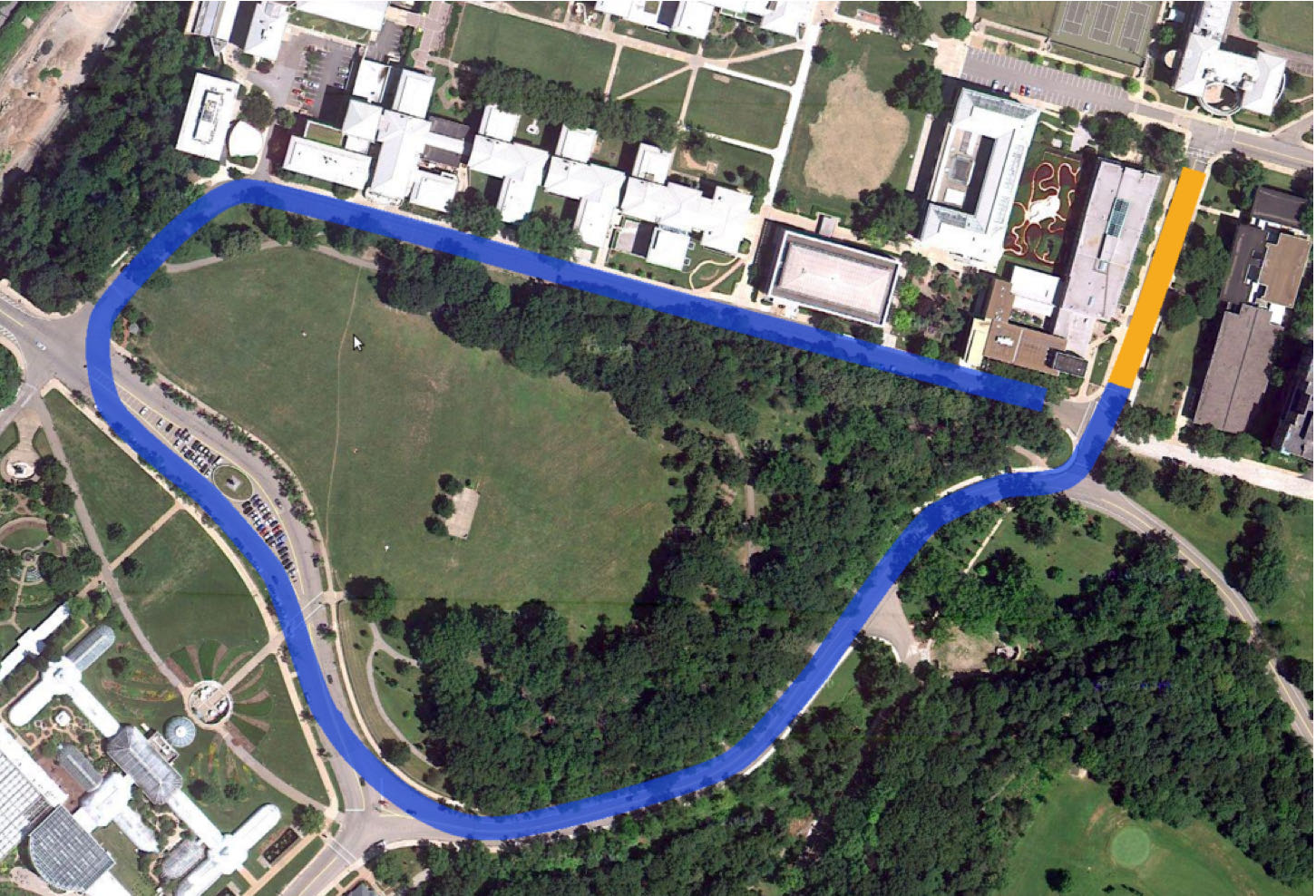
The movement of vehicle is governed by the longitudinal controller and lateral controller. PID is utilized for all longitudinal cases and lateral controller uses different types that will be explained as the following.
PID controller
PID controller functions by tuning the expected value based on calculating the error and using Kp,Ki and Kd together to compute the expexted value, which is summarized by the following equation.
For Longitudinal controller, the error value is computed by calculating the difference between the current speed and desired speed of vehicle.
For Lateral Controller, the error value is computed in a similar way by calculating the difference between the current orientation angle and desired orienatation angle. The desired orienataion angle is calculated using time horizon, i.e. using the current position and future position of the vehicle to determine the curvature.
Pole Placement controller
Pole placement is
a method of calculating the optimum gain matrix used to assign closed-loop poles to specified locations, thereby ensuring system stability
. In this case, the poles are defined as the matrix "poles" that will be utilized to compute the control gain K.
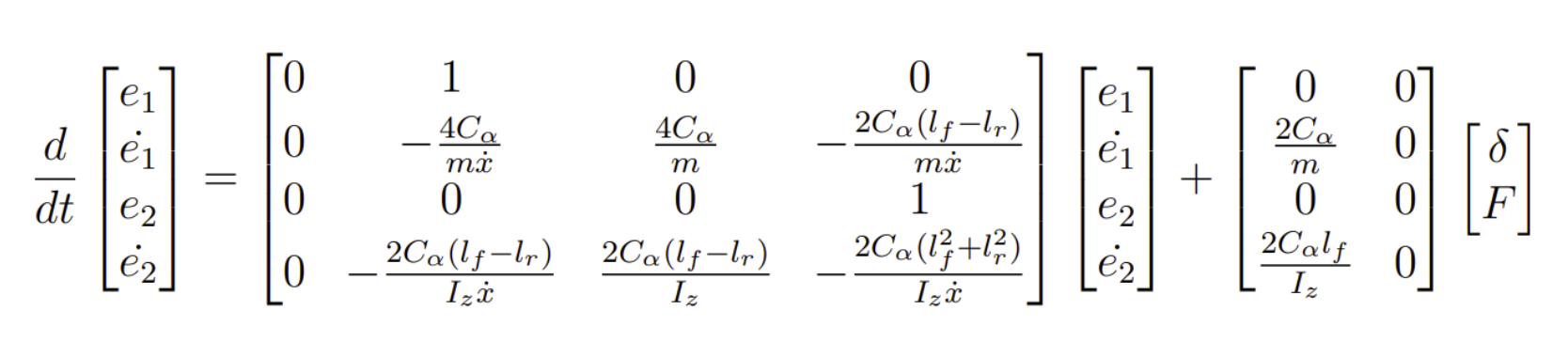
The longitudinal controller is computed using PID. The error for calculating the state space representation of lateral dynamics is shown as the following:
Whereas e1 and e2 the cross-track error, or distance to the center of gravity of the vehicle from the reference trajectory and the heading error, or orientation error of the vehicle with respect to the reference trajectory, respectively.
A and B matrices are constructed based on the state space representation.
The control gain K is computed using K = signal.place_poles(A, B, poles) and passed onto
delta = -(K.gain_matrix @ e) to calculate the desired orientation of the vehicle.
LQR controller
Linear quadratic regulator (LQR) is a widely used method for optimal control of dynamic systems. It can
minimize a cost function that balances the control effort and the deviation from the desired state
.
The same state space representation of error calculation mentioned in the pole placement controller is used for LQR controller.
Given the A and B matrices, C and D matrices can be constructued using a 4x4 identity matrix and 2x4 zeros matrices, respectively. The distretized version of the state space model can be obtained by using signal.cont2discrete(system=(A,B,C,D)). The Q and R matrices are defined and passed to solve matrix S using np.matrix(solve_discrete_are(A_discrete, B_discrete, Q, R)). Finally, the gain matrix K can be computed using the following equation.
The K matrix can then be utilized to calculate the angle error of orientation.
Extended Kalman filter and SLAM
The global coordinates of the Buggy track are given for previous cases. However, in real-life sceanario, this information might to be available and estimate of various values ,e.g. positions and heading angles from observale states need to be computed. The extended Kalman Filter is utilized in this case for predicting the distances to known map coordinates.
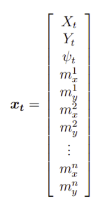
The state vector xt is defined as:
Where subscript m refers to global position and n refers to the number of map features.
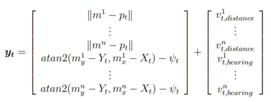
The measurement system yt is defined as the following.
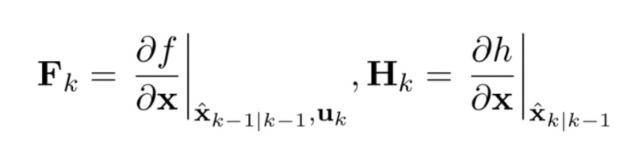
The Jacobian of the predicted state with respect to the previous state, and the Jacobian of the measurement with respect to the state are computed, denoted as F and H and the expressions are shown as the following.
Performance of vehicle in the buggy race track
The performance of the vehicle is evaluated based on the time of completion, maximum deviation from the reference trajectory and average deviation from the reference trajectory. The performances of using different controllers are shown as the following.
| Time of completion (s) | Max. Deviation (m) |
Avg. Deviation (m) |
|
| PID | 400 |
10 | 5 |
| Pole Placement |
350 | 9 | 4.5 |
| LQR | 250 | 7 | 3 |
Extended Kalman Filter Simultaneous Localization and Mapping (EKF SLAM)
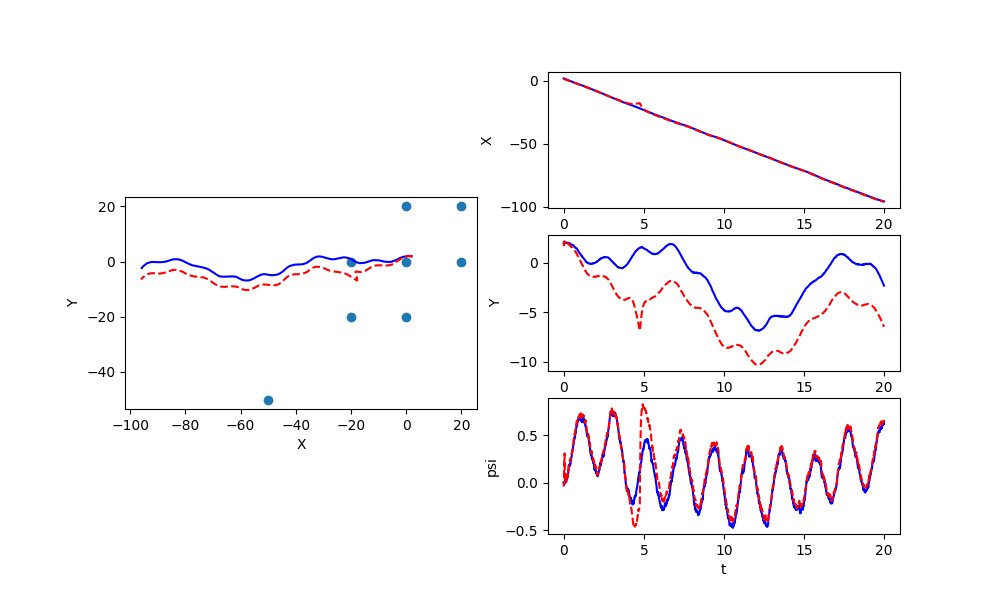
The performance of EKF implementation on an arbitrary trajectory is shown as below.
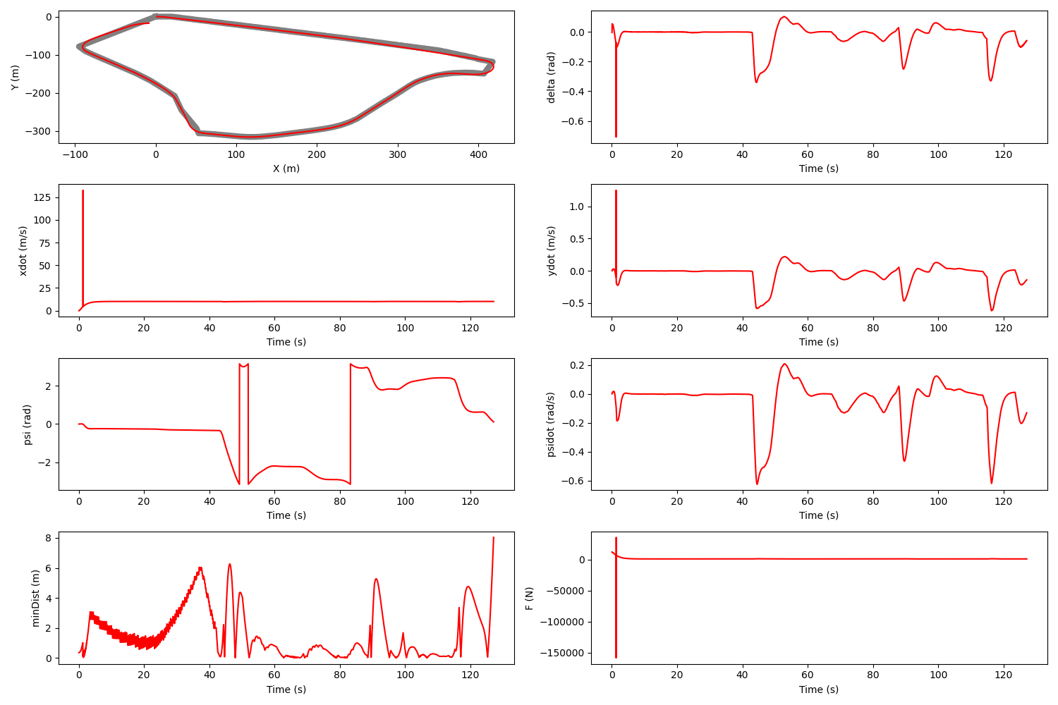
The following plots demonstrate the performance of vehicle integrating EKF implementation and LQR controller on the buggy course.
The performance of tesla model 3 is improved due to iterations of using different types of controllers and the EKF-SLAM enable real-time corrections and environmental updates, helping the vehicle navigate accurately through complex, unfamiliar environments.
This site was created with the Nicepage